Tidy Tuesday Exercise 2

Source

The GitHub repository for TidyTuesday was cloned from https://github.com/rfordatascience/tidytuesday, and the CSV files for 4/11/2023 were copied and pasted into the data folder of this portfolio.

Load Libraries

# Data Handling
library(tidyverse)

Warning: package 'tidyverse' was built under R version 4.2.3

Warning: package 'ggplot2' was built under R version 4.2.3

Warning: package 'tibble' was built under R version 4.2.3

Warning: package 'tidyr' was built under R version 4.2.3

Warning: package 'readr' was built under R version 4.2.3

Warning: package 'dplyr' was built under R version 4.2.3

Warning: package 'forcats' was built under R version 4.2.3

Warning: package 'lubridate' was built under R version 4.2.3

── Attaching core tidyverse packages ──────────────────────── tidyverse 2.0.0 ──
✔ dplyr     1.1.1     ✔ readr     2.1.4
✔ forcats   1.0.0     ✔ stringr   1.5.0
✔ ggplot2   3.4.1     ✔ tibble    3.2.1
✔ lubridate 1.9.2     ✔ tidyr     1.3.0
✔ purrr     1.0.1     
── Conflicts ────────────────────────────────────────── tidyverse_conflicts() ──
✖ dplyr::filter() masks stats::filter()
✖ dplyr::lag()    masks stats::lag()
ℹ Use the conflicted package (<http://conflicted.r-lib.org/>) to force all conflicts to become errors

## Information About NAs
library(dlookr)

Attaching package: 'dlookr'

The following object is masked from 'package:tidyr':

    extract

The following object is masked from 'package:base':

    transform

# Model Handling
library(tidymodels)

── Attaching packages ────────────────────────────────────── tidymodels 1.0.0 ──
✔ broom        1.0.4     ✔ rsample      1.1.1
✔ dials        1.1.0     ✔ tune         1.0.1
✔ infer        1.0.4     ✔ workflows    1.1.3
✔ modeldata    1.1.0     ✔ workflowsets 1.0.0
✔ parsnip      1.0.4     ✔ yardstick    1.1.0
✔ recipes      1.0.5     

Warning: package 'broom' was built under R version 4.2.3

Warning: package 'modeldata' was built under R version 4.2.3

Warning: package 'parsnip' was built under R version 4.2.3

Warning: package 'recipes' was built under R version 4.2.3

Warning: package 'workflows' was built under R version 4.2.3

── Conflicts ───────────────────────────────────────── tidymodels_conflicts() ──
✖ scales::discard() masks purrr::discard()
✖ dlookr::extract() masks tidyr::extract()
✖ dplyr::filter()   masks stats::filter()
✖ recipes::fixed()  masks stringr::fixed()
✖ dplyr::lag()      masks stats::lag()
✖ yardstick::spec() masks readr::spec()
✖ recipes::step()   masks stats::step()
• Learn how to get started at https://www.tidymodels.org/start/

library(rpart)

Attaching package: 'rpart'

The following object is masked from 'package:dials':

    prune

Load Data

# First Dataset
cage_free_data <- read_csv("data/cage-free-percentages.csv")

Rows: 96 Columns: 4
── Column specification ────────────────────────────────────────────────────────
Delimiter: ","
chr  (1): source
dbl  (2): percent_hens, percent_eggs
date (1): observed_month

ℹ Use `spec()` to retrieve the full column specification for this data.
ℹ Specify the column types or set `show_col_types = FALSE` to quiet this message.

# Second Dataset
egg_production_data <- read_csv("data/egg-production.csv")

Rows: 220 Columns: 6
── Column specification ────────────────────────────────────────────────────────
Delimiter: ","
chr  (3): prod_type, prod_process, source
dbl  (2): n_hens, n_eggs
date (1): observed_month

ℹ Use `spec()` to retrieve the full column specification for this data.
ℹ Specify the column types or set `show_col_types = FALSE` to quiet this message.

Explore Data

# Cage-Free Eggs
str(cage_free_data)

spc_tbl_ [96 × 4] (S3: spec_tbl_df/tbl_df/tbl/data.frame)
 $ observed_month: Date[1:96], format: "2007-12-31" "2008-12-31" ...
 $ percent_hens  : num [1:96] 3.2 3.5 3.6 4.4 5.4 6 5.9 5.7 8.6 9.9 ...
 $ percent_eggs  : num [1:96] NA NA NA NA NA NA NA NA NA NA ...
 $ source        : chr [1:96] "Egg-Markets-Overview-2019-10-19.pdf" "Egg-Markets-Overview-2019-10-19.pdf" "Egg-Markets-Overview-2019-10-19.pdf" "Egg-Markets-Overview-2019-10-19.pdf" ...
 - attr(*, "spec")=
  .. cols(
  ..   observed_month = col_date(format = ""),
  ..   percent_hens = col_double(),
  ..   percent_eggs = col_double(),
  ..   source = col_character()
  .. )
 - attr(*, "problems")=<externalptr> 

summary(cage_free_data)

 observed_month        percent_hens    percent_eggs       source         
 Min.   :2007-12-31   Min.   : 3.20   Min.   : 9.557   Length:96         
 1st Qu.:2017-05-23   1st Qu.:13.46   1st Qu.:14.521   Class :character  
 Median :2018-11-15   Median :17.30   Median :16.235   Mode  :character  
 Mean   :2018-05-12   Mean   :17.95   Mean   :17.095                     
 3rd Qu.:2020-02-28   3rd Qu.:23.46   3rd Qu.:19.460                     
 Max.   :2021-02-28   Max.   :29.20   Max.   :24.546                     
                                      NA's   :42                         

head(cage_free_data)

# A tibble: 6 × 4
  observed_month percent_hens percent_eggs source                             
  <date>                <dbl>        <dbl> <chr>                              
1 2007-12-31              3.2           NA Egg-Markets-Overview-2019-10-19.pdf
2 2008-12-31              3.5           NA Egg-Markets-Overview-2019-10-19.pdf
3 2009-12-31              3.6           NA Egg-Markets-Overview-2019-10-19.pdf
4 2010-12-31              4.4           NA Egg-Markets-Overview-2019-10-19.pdf
5 2011-12-31              5.4           NA Egg-Markets-Overview-2019-10-19.pdf
6 2012-12-31              6             NA Egg-Markets-Overview-2019-10-19.pdf

plot_na_pareto(cage_free_data)

# Egg Production
str(egg_production_data)

spc_tbl_ [220 × 6] (S3: spec_tbl_df/tbl_df/tbl/data.frame)
 $ observed_month: Date[1:220], format: "2016-07-31" "2016-08-31" ...
 $ prod_type     : chr [1:220] "hatching eggs" "hatching eggs" "hatching eggs" "hatching eggs" ...
 $ prod_process  : chr [1:220] "all" "all" "all" "all" ...
 $ n_hens        : num [1:220] 57975000 57595000 57161000 56857000 57116000 ...
 $ n_eggs        : num [1:220] 1.15e+09 1.14e+09 1.09e+09 1.13e+09 1.10e+09 ...
 $ source        : chr [1:220] "ChicEggs-09-23-2016.pdf" "ChicEggs-10-21-2016.pdf" "ChicEggs-11-22-2016.pdf" "ChicEggs-12-23-2016.pdf" ...
 - attr(*, "spec")=
  .. cols(
  ..   observed_month = col_date(format = ""),
  ..   prod_type = col_character(),
  ..   prod_process = col_character(),
  ..   n_hens = col_double(),
  ..   n_eggs = col_double(),
  ..   source = col_character()
  .. )
 - attr(*, "problems")=<externalptr> 

summary(egg_production_data)

 observed_month        prod_type         prod_process           n_hens         
 Min.   :2016-07-31   Length:220         Length:220         Min.   : 13500000  
 1st Qu.:2017-09-30   Class :character   Class :character   1st Qu.: 17284500  
 Median :2018-11-15   Mode  :character   Mode  :character   Median : 59939500  
 Mean   :2018-11-14                                         Mean   :110839873  
 3rd Qu.:2019-12-31                                         3rd Qu.:125539250  
 Max.   :2021-02-28                                         Max.   :341166000  
     n_eggs             source         
 Min.   :2.981e+08   Length:220        
 1st Qu.:4.240e+08   Class :character  
 Median :1.155e+09   Mode  :character  
 Mean   :2.607e+09                     
 3rd Qu.:2.963e+09                     
 Max.   :8.601e+09                     

head(egg_production_data)

# A tibble: 6 × 6
  observed_month prod_type     prod_process   n_hens     n_eggs source          
  <date>         <chr>         <chr>           <dbl>      <dbl> <chr>           
1 2016-07-31     hatching eggs all          57975000 1147000000 ChicEggs-09-23-…
2 2016-08-31     hatching eggs all          57595000 1142700000 ChicEggs-10-21-…
3 2016-09-30     hatching eggs all          57161000 1093300000 ChicEggs-11-22-…
4 2016-10-31     hatching eggs all          56857000 1126700000 ChicEggs-12-23-…
5 2016-11-30     hatching eggs all          57116000 1096600000 ChicEggs-01-24-…
6 2016-12-31     hatching eggs all          57750000 1132900000 ChicEggs-02-28-…

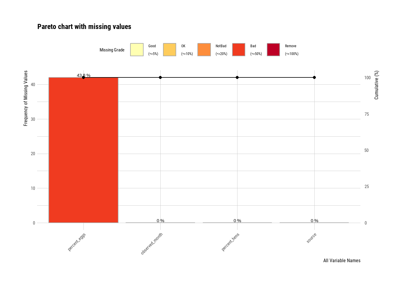
# plot_na_pareto(egg_production_data) <-- Was edited out since no NA values were found for this dataset.

Question(s) and Hypothesis

Upon reviewing the datasets, two questions have come to mind:

• Is there a month in which more eggs are produced than others?

• Have the percentages of cage-free hens and eggs increased over time?

The hypotheses are therefore:

• August sees the greatest production of eggs in general.

• The percentages of cage-free hens and eggs have increased through the years.

Data Cleaning, Manipulation, and Processing

The data given by TidyTuesday appears mostly clean already, though it would probably be better to combine the two datasets into one during data cleaning/manipulation. According to the README, the cage-free data refers to what percent of hens and eggs out of all the production facilities in the United States are cage-free. It is therefore likely that the information in cage_free_data is already contained in egg_production_data in some way.

The two datasets also begin at different points in time, so we will choose the dataset that starts more recently (aka egg_production_data). Furthermore, since observed month comes in sets of 2, that makes it relatively easy to calculate total number of hens and eggs for each month indicated.

Make Column for Month

egg_production_data <- egg_production_data %>%
  mutate(Month = month(ymd(observed_month))) %>%
  mutate(character_month = case_when(
    Month == 1 ~ "January",
    Month == 2 ~ "February",
    Month == 3 ~ "March",
    Month == 4 ~ "April",
    Month == 5 ~ "May",
    Month == 6 ~ "June",
    Month == 7 ~ "July",
    Month == 8 ~ "August",
    Month == 9 ~ "September",
    Month == 10 ~ "October",
    Month == 11 ~ "November",
    Month == 12 ~ "December"))

egg_production_data$character_month <- factor(egg_production_data$character_month, levels = c("January", "February", "March", "April", "May", "June", "July", "August", "September", "October", "November", "December"), ordered = TRUE)

Calculate Total Eggs Produced Each Month

# Have Columns to Refer Back to Previous/Next Entries
compatible_egg_production_data <- egg_production_data %>%
  arrange(observed_month) %>%
  mutate(previous_n_hens = lag(n_hens, n = 1)) %>%
  mutate(previous_n_eggs = lag(n_eggs, n = 1)) %>%
  mutate(proximo_n_hens = lead(n_hens, n = 1)) %>%
  mutate(proximo_n_eggs = lead(n_eggs, n = 1))

# Calculate Total Number of Hens and Eggs Based on Row Divisibility (Each Month Appears Twice)
row_EO <- NA
for (row in 1:nrow(compatible_egg_production_data)) {
  row_EO <- c(row_EO, row)
}
row_EO <- row_EO[2:221]
compatible_egg_production_data$row_EO <- row_EO

compatible_egg_production_data <- compatible_egg_production_data %>%
  mutate(total_n_hens = case_when(
    row_EO %% 2 == 0 ~ n_hens + previous_n_hens,
    TRUE ~ n_hens + proximo_n_hens)) %>%
  mutate(total_n_eggs = case_when(
    row_EO %% 2 == 0 ~ n_eggs + previous_n_eggs,
    TRUE ~ n_eggs + proximo_n_eggs))

Data Visualization

Production of Eggs by Month

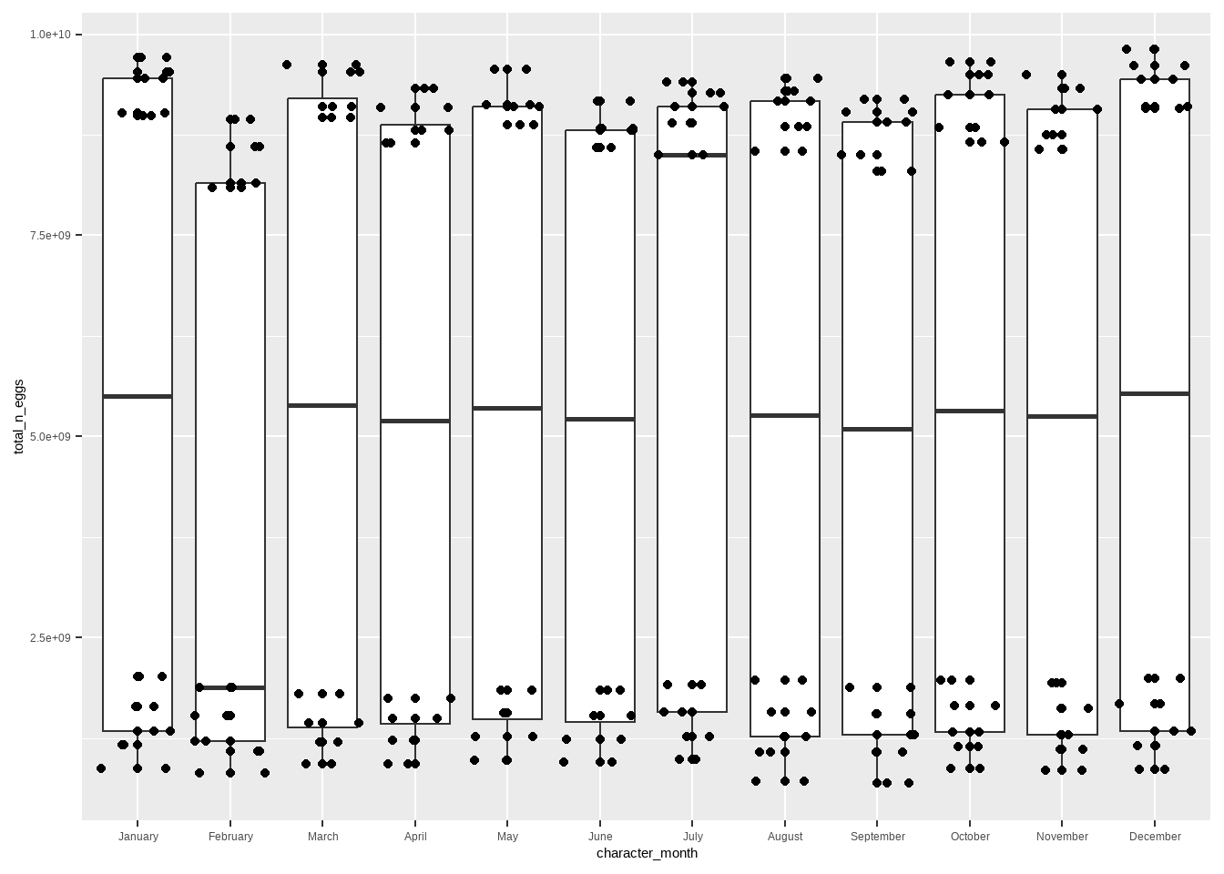
ggplot(compatible_egg_production_data, aes(x = character_month, y = total_n_eggs)) + geom_boxplot() + geom_point() + geom_jitter()

It appears that August is not when the most eggs are produced; rather, most eggs are produced in January and December, though it is noteworthy that July has a very high median of egg production in comparison to other months.

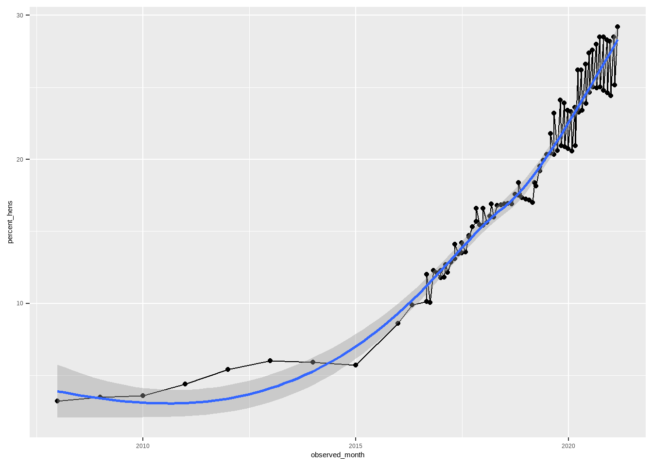
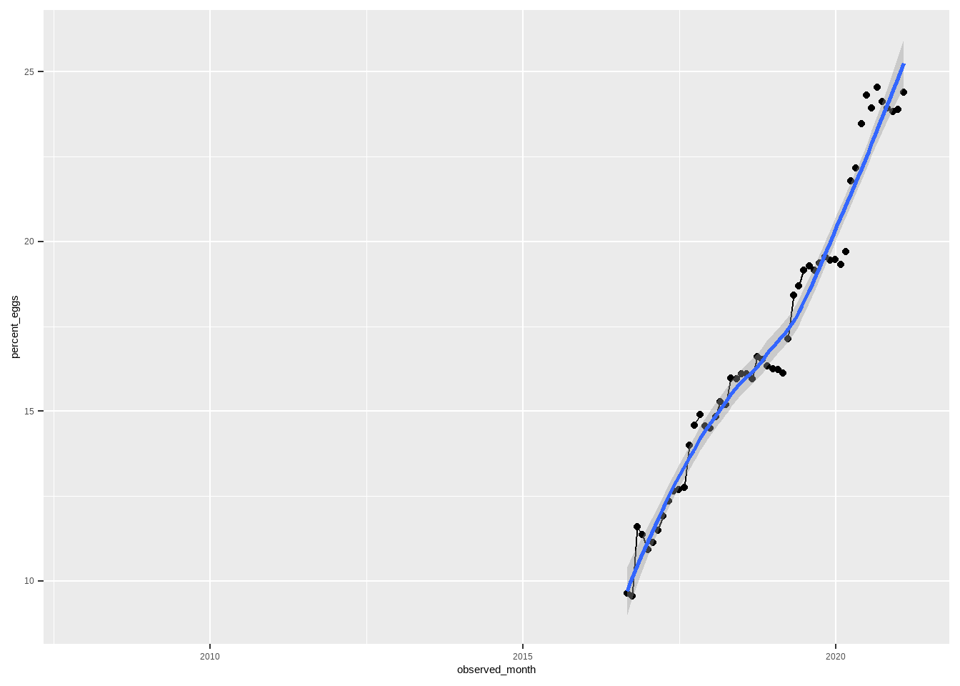
Change in Percentage of Cage-Free Hens/Eggs Over Time

# Hens
ggplot(cage_free_data %>% arrange(observed_month), aes(x = observed_month, y = percent_hens)) + geom_point() + geom_line() + geom_smooth()

`geom_smooth()` using method = 'loess' and formula = 'y ~ x'

# Eggs
ggplot(cage_free_data %>% arrange(observed_month), aes(x = observed_month, y = percent_eggs)) + geom_point() + geom_line() + geom_smooth()

`geom_smooth()` using method = 'loess' and formula = 'y ~ x'

Warning: Removed 42 rows containing non-finite values (`stat_smooth()`).

Warning: Removed 42 rows containing missing values (`geom_point()`).

Warning: Removed 11 rows containing missing values (`geom_line()`).

It appears that the percentage of cage-free eggs has increased dramatically over time.

Machine Learning

At this point, I would like to see machine learning models for linear regression, tree, random forest, and LASSO to predict egg count and compare its performance on “training” data to “test” data.

Setup

# Choose Predictors of Interest and Outcomes
egg_production_data <- egg_production_data %>% select(!c("observed_month", "source", "character_month"))

# Reproducibility
set.seed(123)

# Split Egg Production Data
data_division <- initial_split(egg_production_data, prop = 7/10)
train_data <- training(data_division)
test_data <- testing(data_division)

post_cv <- vfold_cv(train_data)

# Recipe
egg_recipe <- recipe(n_eggs ~ ., data = train_data)

# Workflow
## Linear Model
linear_model <- linear_reg() %>% set_engine("lm")
linear_workflow <- workflow() %>%
  add_model(linear_model) %>%
  add_recipe(egg_recipe)

## Tree Model
tree_model <- decision_tree(cost_complexity = tune(), tree_depth = tune()) %>% set_engine("rpart") %>% set_mode("regression")
tree_grid <- grid_regular(
  cost_complexity(),
  tree_depth(),
  levels = 5
)
tree_workflow <- workflow() %>%
  add_model(tree_model) %>%
  add_formula(n_eggs ~ .)

## Random Forest
random_forest_model <- rand_forest(mtry = tune(), min_n = tune(), trees = 1000) %>%
  set_engine("ranger", importance = 'impurity') %>%
  set_mode("regression")
random_forest_workflow <- workflow() %>%
  add_recipe(egg_recipe) %>%
  add_model(random_forest_model)

## LASSO
lasso_model <- linear_reg(penalty = tune(), mixture = 1) %>% set_engine("glmnet")
lasso_workflow <- workflow() %>% add_model(lasso_model) %>% add_formula(n_eggs ~ .)
lasso_grid <- tibble(penalty = 10^seq(-4, -1, length.out = 30))

Fitting

# Linear Model
fit_linear <- linear_workflow %>% fit(train_data)
fit_linear %>% extract_fit_parsnip() %>% tidy()

# A tibble: 6 × 5
  term                                    estimate  std.error statistic  p.value
  <chr>                                      <dbl>      <dbl>     <dbl>    <dbl>
1 (Intercept)                         -455404907.      8.96e7    -5.08  1.11e- 6
2 prod_typetable eggs                   69469257.      3.44e8     0.202 8.40e- 1
3 prod_processcage-free (non-organic)  239893321.      3.70e8     0.648 5.18e- 1
4 prod_processcage-free (organic)      297180705.      4.05e8     0.734 4.64e- 1
5 n_hens                                      25.4     1.31e0    19.4   1.68e-42
6 Month                                  8538855.      3.21e6     2.66  8.68e- 3

linear_augment <- augment(fit_linear, train_data)
linear_augment %>% select(n_eggs, .pred) %>% rmse(n_eggs, .pred)

# A tibble: 1 × 3
  .metric .estimator  .estimate
  <chr>   <chr>           <dbl>
1 rmse    standard   133763971.

## RMSE: 133763971

# Tree Model
tree_tuned <- tree_workflow %>%
  tune_grid(resamples = post_cv, grid = tree_grid)
tree_tuned %>% collect_metrics()

# A tibble: 50 × 8
   cost_complexity tree_depth .metric .estimator      mean     n std_err .config
             <dbl>      <int> <chr>   <chr>          <dbl> <int>   <dbl> <chr>  
 1    0.0000000001          1 rmse    standard     3.96e+8    10 1.27e+7 Prepro…
 2    0.0000000001          1 rsq     standard     9.81e-1    10 4.79e-3 Prepro…
 3    0.0000000178          1 rmse    standard     3.96e+8    10 1.27e+7 Prepro…
 4    0.0000000178          1 rsq     standard     9.81e-1    10 4.79e-3 Prepro…
 5    0.00000316            1 rmse    standard     3.96e+8    10 1.27e+7 Prepro…
 6    0.00000316            1 rsq     standard     9.81e-1    10 4.79e-3 Prepro…
 7    0.000562              1 rmse    standard     3.96e+8    10 1.27e+7 Prepro…
 8    0.000562              1 rsq     standard     9.81e-1    10 4.79e-3 Prepro…
 9    0.1                   1 rmse    standard     3.96e+8    10 1.27e+7 Prepro…
10    0.1                   1 rsq     standard     9.81e-1    10 4.79e-3 Prepro…
# ℹ 40 more rows

tree_tuned %>% show_best(metric = "rmse") %>% arrange(mean)

# A tibble: 5 × 8
  cost_complexity tree_depth .metric .estimator       mean     n std_err .config
            <dbl>      <int> <chr>   <chr>           <dbl> <int>   <dbl> <chr>  
1    0.0000000001          8 rmse    standard   174031309.    10  1.42e7 Prepro…
2    0.0000000178          8 rmse    standard   174031309.    10  1.42e7 Prepro…
3    0.00000316            8 rmse    standard   174031309.    10  1.42e7 Prepro…
4    0.0000000001         11 rmse    standard   174031309.    10  1.42e7 Prepro…
5    0.0000000178         11 rmse    standard   174031309.    10  1.42e7 Prepro…

best_tree <- tree_tuned %>% select_best(metric = "rmse")
best_tree

# A tibble: 1 × 3
  cost_complexity tree_depth .config              
            <dbl>      <int> <chr>                
1    0.0000000001          8 Preprocessor1_Model11

## RMSE: 174031309

# Random Forest
doParallel::registerDoParallel()
random_forest_tuned <- random_forest_workflow %>%
  tune_grid(
    resamples = post_cv,
    grid = 15,
    control = control_grid(save_pred = TRUE),
    metrics = metric_set(rmse)
  )

i Creating pre-processing data to finalize unknown parameter: mtry

random_forest_tuned %>% show_best(metric = "rmse")

# A tibble: 5 × 8
   mtry min_n .metric .estimator       mean     n   std_err .config             
  <int> <int> <chr>   <chr>           <dbl> <int>     <dbl> <chr>               
1     3     5 rmse    standard   150855368.    10 17578066. Preprocessor1_Model…
2     3     2 rmse    standard   152178259.    10 17542732. Preprocessor1_Model…
3     3    11 rmse    standard   153738405.    10 16189038. Preprocessor1_Model…
4     4    14 rmse    standard   161256511.    10 16141692. Preprocessor1_Model…
5     2     7 rmse    standard   162101309.    10 15680177. Preprocessor1_Model…

best_random_forest <- random_forest_tuned %>% select_best(metric = "rmse")

## RMSE: 150855368

# LASSO
lasso_tuned <- lasso_workflow %>% 
  tune_grid(resamples = post_cv, 
            grid = lasso_grid, 
            control = control_grid(verbose = FALSE, save_pred = TRUE),
            metrics = metric_set(rmse))

lasso_tuned %>% collect_metrics()

# A tibble: 30 × 7
    penalty .metric .estimator       mean     n   std_err .config              
      <dbl> <chr>   <chr>           <dbl> <int>     <dbl> <chr>                
 1 0.0001   rmse    standard   127279088.    10 18202748. Preprocessor1_Model01
 2 0.000127 rmse    standard   127279088.    10 18202748. Preprocessor1_Model02
 3 0.000161 rmse    standard   127279088.    10 18202748. Preprocessor1_Model03
 4 0.000204 rmse    standard   127279088.    10 18202748. Preprocessor1_Model04
 5 0.000259 rmse    standard   127279088.    10 18202748. Preprocessor1_Model05
 6 0.000329 rmse    standard   127279088.    10 18202748. Preprocessor1_Model06
 7 0.000418 rmse    standard   127279088.    10 18202748. Preprocessor1_Model07
 8 0.000530 rmse    standard   127279088.    10 18202748. Preprocessor1_Model08
 9 0.000672 rmse    standard   127279088.    10 18202748. Preprocessor1_Model09
10 0.000853 rmse    standard   127279088.    10 18202748. Preprocessor1_Model10
# ℹ 20 more rows

lasso_tuned %>% show_best("rmse")

# A tibble: 5 × 7
   penalty .metric .estimator       mean     n   std_err .config              
     <dbl> <chr>   <chr>           <dbl> <int>     <dbl> <chr>                
1 0.0001   rmse    standard   127279088.    10 18202748. Preprocessor1_Model01
2 0.000127 rmse    standard   127279088.    10 18202748. Preprocessor1_Model02
3 0.000161 rmse    standard   127279088.    10 18202748. Preprocessor1_Model03
4 0.000204 rmse    standard   127279088.    10 18202748. Preprocessor1_Model04
5 0.000259 rmse    standard   127279088.    10 18202748. Preprocessor1_Model05

lasso_best <- lasso_tuned %>% select_best("rmse")

## RMSE: 127279088

Evaluation

Based on the above, the LASSO model performed the best with the lowest RMSE.

final_workflow <- lasso_workflow %>% finalize_workflow(lasso_best)
final_workflow %>% fit(train_data) %>% extract_fit_parsnip() %>% tidy()

Warning: package 'glmnet' was built under R version 4.2.3

Loading required package: Matrix

Attaching package: 'Matrix'

The following objects are masked from 'package:tidyr':

    expand, pack, unpack

Loaded glmnet 4.1-7

# A tibble: 6 × 3
  term                                    estimate penalty
  <chr>                                      <dbl>   <dbl>
1 (Intercept)                         -344068420.   0.0001
2 prod_typetable eggs                  283388358.   0.0001
3 prod_processcage-free (non-organic)          0    0.0001
4 prod_processcage-free (organic)              0    0.0001
5 n_hens                                      24.4  0.0001
6 Month                                  4468627.   0.0001

final_workflow %>% fit(train_data) %>% augment(train_data) %>% rmse(n_eggs, .pred)

# A tibble: 1 × 3
  .metric .estimator  .estimate
  <chr>   <chr>           <dbl>
1 rmse    standard   135992484.

# RMSE for Training Data: 135992484

final_workflow %>% fit(test_data) %>% extract_fit_parsnip() %>% tidy()

# A tibble: 6 × 3
  term                                    estimate penalty
  <chr>                                      <dbl>   <dbl>
1 (Intercept)                         -281435860.   0.0001
2 prod_typetable eggs                  242458856.   0.0001
3 prod_processcage-free (non-organic)          0    0.0001
4 prod_processcage-free (organic)              0    0.0001
5 n_hens                                      24.5  0.0001
6 Month                                        0    0.0001

final_workflow %>% fit(test_data) %>% augment(test_data) %>% rmse(n_eggs, .pred)

# A tibble: 1 × 3
  .metric .estimator .estimate
  <chr>   <chr>          <dbl>
1 rmse    standard   89508484.

# RMSE for Testing Data: 89508484

It is slightly surprising to me that the LASSO model performs better on the testing data than on the training data.

Discussion

From this analysis, the hypothesis that August is the month of highest egg production has been proved false. However, the hypothesis that percentage of cage-free hens and eggs increasing over time appears to be confirmed. While none of the models fitted to the training data had a low RMSE, the LASSO model had the lowest of them and performed better on the testing data than on the training data.