Module 8 Exercise - Fitting Basic Statistical Models: Part 2

Setup

Tidyverse will be used for graphing in addition to handling data processing/manipulation, and the here package assists in pathing.

Load Required R Packages

Load Cleaned Data

# Pathing
data_path <- here("fluanalysis", "data", "cleaned_data.rds")

# Data Importation
clean_data <- readRDS(data_path)

Exploratory Data Analysis

To get a greater sense of the dataset’s structure, I’ll run the str() command and determine which variables of interest are numeric and/or continuous.

Data Structure

str(clean_data)

'data.frame':   730 obs. of  32 variables:
 $ SwollenLymphNodes: Factor w/ 2 levels "No","Yes": 2 2 2 2 2 1 1 1 2 1 ...
  ..- attr(*, "label")= chr "Swollen Lymph Nodes"
 $ ChestCongestion  : Factor w/ 2 levels "No","Yes": 1 2 2 2 1 1 1 2 2 2 ...
  ..- attr(*, "label")= chr "Chest Congestion"
 $ ChillsSweats     : Factor w/ 2 levels "No","Yes": 1 1 2 2 2 2 2 2 2 1 ...
  ..- attr(*, "label")= chr "Chills/Sweats"
 $ NasalCongestion  : Factor w/ 2 levels "No","Yes": 1 2 2 2 1 1 1 2 2 2 ...
  ..- attr(*, "label")= chr "Nasal Congestion"
 $ CoughYN          : Factor w/ 2 levels "No","Yes": 2 2 1 2 1 2 2 2 2 2 ...
  ..- attr(*, "label")= chr "Cough"
 $ Sneeze           : Factor w/ 2 levels "No","Yes": 1 1 2 2 1 2 1 2 1 1 ...
  ..- attr(*, "label")= chr "Sneeze"
 $ Fatigue          : Factor w/ 2 levels "No","Yes": 2 2 2 2 2 2 2 2 2 2 ...
  ..- attr(*, "label")= chr "Fatigue"
 $ SubjectiveFever  : Factor w/ 2 levels "No","Yes": 2 2 2 2 2 2 2 2 2 1 ...
  ..- attr(*, "label")= chr "Subjective Fever"
 $ Headache         : Factor w/ 2 levels "No","Yes": 2 2 2 2 2 2 1 2 2 2 ...
  ..- attr(*, "label")= chr "Headache"
 $ Weakness         : Factor w/ 4 levels "None","Mild",..: 2 4 4 4 3 3 2 4 3 3 ...
 $ WeaknessYN       : Factor w/ 2 levels "No","Yes": 2 2 2 2 2 2 2 2 2 2 ...
  ..- attr(*, "label")= chr "Weakness"
 $ CoughIntensity   : Factor w/ 4 levels "None","Mild",..: 4 4 2 3 1 3 4 3 3 3 ...
  ..- attr(*, "label")= chr "Cough Severity"
 $ CoughYN2         : Factor w/ 2 levels "No","Yes": 2 2 2 2 1 2 2 2 2 2 ...
 $ Myalgia          : Factor w/ 4 levels "None","Mild",..: 2 4 4 4 2 3 2 4 3 2 ...
 $ MyalgiaYN        : Factor w/ 2 levels "No","Yes": 2 2 2 2 2 2 2 2 2 2 ...
  ..- attr(*, "label")= chr "Myalgia"
 $ RunnyNose        : Factor w/ 2 levels "No","Yes": 1 1 2 2 1 1 2 2 2 2 ...
  ..- attr(*, "label")= chr "Runny Nose"
 $ AbPain           : Factor w/ 2 levels "No","Yes": 1 1 2 1 1 1 1 1 1 1 ...
  ..- attr(*, "label")= chr "Abdominal Pain"
 $ ChestPain        : Factor w/ 2 levels "No","Yes": 1 1 2 1 1 2 2 1 1 1 ...
  ..- attr(*, "label")= chr "Chest Pain"
 $ Diarrhea         : Factor w/ 2 levels "No","Yes": 1 1 1 1 1 2 1 1 1 1 ...
 $ EyePn            : Factor w/ 2 levels "No","Yes": 1 1 1 1 2 1 1 1 1 1 ...
  ..- attr(*, "label")= chr "Eye Pain"
 $ Insomnia         : Factor w/ 2 levels "No","Yes": 1 1 2 2 2 1 1 2 2 2 ...
  ..- attr(*, "label")= chr "Sleeplessness"
 $ ItchyEye         : Factor w/ 2 levels "No","Yes": 1 1 1 1 1 1 1 1 1 1 ...
  ..- attr(*, "label")= chr "Itchy Eyes"
 $ Nausea           : Factor w/ 2 levels "No","Yes": 1 1 2 2 2 2 1 1 2 2 ...
 $ EarPn            : Factor w/ 2 levels "No","Yes": 1 2 1 2 1 1 1 1 1 1 ...
  ..- attr(*, "label")= chr "Ear Pain"
 $ Hearing          : Factor w/ 2 levels "No","Yes": 1 2 1 1 1 1 1 1 1 1 ...
  ..- attr(*, "label")= chr "Loss of Hearing"
 $ Pharyngitis      : Factor w/ 2 levels "No","Yes": 2 2 2 2 2 2 2 1 1 1 ...
  ..- attr(*, "label")= chr "Sore Throat"
 $ Breathless       : Factor w/ 2 levels "No","Yes": 1 1 2 1 1 2 1 1 1 2 ...
  ..- attr(*, "label")= chr "Breathlessness"
 $ ToothPn          : Factor w/ 2 levels "No","Yes": 1 1 2 1 1 1 1 1 2 1 ...
  ..- attr(*, "label")= chr "Tooth Pain"
 $ Vision           : Factor w/ 2 levels "No","Yes": 1 1 1 1 1 1 1 1 1 1 ...
  ..- attr(*, "label")= chr "Blurred Vision"
 $ Vomit            : Factor w/ 2 levels "No","Yes": 1 1 1 1 1 1 2 1 1 1 ...
  ..- attr(*, "label")= chr "Vomiting"
 $ Wheeze           : Factor w/ 2 levels "No","Yes": 1 1 1 2 1 2 1 1 1 1 ...
  ..- attr(*, "label")= chr "Wheezing"
 $ BodyTemp         : num  98.3 100.4 100.8 98.8 100.5 ...

It appears that there is only one numeric/continuous variable: BodyTemp. BodyTemp will also serve as the main continuous outcome of interest, and Nausea will serve as the main categorical outcome.

Categorical Variables

Categorical variables include: SwollenLymphNodes, ChestCongestion, ChillsSweats, NasalCongestion, CoughYN, Sneeze, Fatigue, Subjective Fever, Headache, Weakness, WeaknessYN, CoughIntensity, CoughYN2, Myalgia, MyalgiaYN, RunnyNose, AbPain, ChestPain, Diarrhea, EyePn, Insomnia, ItchyEye, Nausea, EarPn, Hearing, Pharyngitis, Breathless, ToothPn, Vision, Vomit, and Wheeze.

Since these categorical variables are just Y/N, the number of yes/no’s will be presented in a table for each.

Main Categorical Outcome - Nausea

# Table
rmarkdown::paged_table(clean_data %>% group_by(Nausea) %>% count())

Other Categorical Variables (Predictors)

# Swollen Lymph Nodes
rmarkdown::paged_table(clean_data %>% group_by(SwollenLymphNodes) %>% count())

# Chest Congestion and Chest Pain
## Congestion
rmarkdown::paged_table(clean_data %>% group_by(ChestCongestion) %>% count())

## Pain
rmarkdown::paged_table(clean_data %>% group_by(ChestPain) %>% count())

# Chills/Sweats
rmarkdown::paged_table(clean_data %>% group_by(ChillsSweats) %>% count())

# Nasal Congestion
rmarkdown::paged_table(clean_data %>% group_by(NasalCongestion) %>% count())

# Coughing
## Y/N
rmarkdown::paged_table(clean_data %>% group_by(CoughYN) %>% count())

## Intensity
rmarkdown::paged_table(clean_data %>% group_by(CoughIntensity) %>% count())

## 2nd Y/N
rmarkdown::paged_table(clean_data %>% group_by(CoughYN2) %>% count())

# Sneezing
rmarkdown::paged_table(clean_data %>% group_by(Sneeze) %>% count())

# Fatigue
rmarkdown::paged_table(clean_data %>% group_by(Fatigue) %>% count())

# Subjective Fever
rmarkdown::paged_table(clean_data %>% group_by(SubjectiveFever) %>% count())

# Headache
rmarkdown::paged_table(clean_data %>% group_by(Headache) %>% count())

# Weakness
## Severity
rmarkdown::paged_table(clean_data %>% group_by(Weakness) %>% count())

## Y/N
rmarkdown::paged_table(clean_data %>% group_by(WeaknessYN) %>% count())

# Myalgia
## Y/N
rmarkdown::paged_table(clean_data %>% group_by(MyalgiaYN) %>% count())

## Severity
rmarkdown::paged_table(clean_data %>% group_by(Myalgia) %>% count())

# Runny Nose
rmarkdown::paged_table(clean_data %>% group_by(RunnyNose) %>% count())

# Abdominal Pain
rmarkdown::paged_table(clean_data %>% group_by(AbPain) %>% count())

# Diarrhea
rmarkdown::paged_table(clean_data %>% group_by(Diarrhea) %>% count())

# Eye/Vision
## Pain
rmarkdown::paged_table(clean_data %>% group_by(EyePn) %>% count())

## Itchyness
rmarkdown::paged_table(clean_data %>% group_by(ItchyEye) %>% count())

## Vision
rmarkdown::paged_table(clean_data %>% group_by(Vision) %>% count())

# Insomnia
rmarkdown::paged_table(clean_data %>% group_by(Insomnia) %>% count())

# Ear/Hearing
## Pain
rmarkdown::paged_table(clean_data %>% group_by(EarPn) %>% count())

## Hearing
rmarkdown::paged_table(clean_data %>% group_by(Hearing) %>% count())

# Pharyngitis
rmarkdown::paged_table(clean_data %>% group_by(Pharyngitis) %>% count())

# Breathless/Wheezing
## Breathless
rmarkdown::paged_table(clean_data %>% group_by(Breathless) %>% count())

## Wheezing
rmarkdown::paged_table(clean_data %>% group_by(Wheeze) %>% count())

# Tooth Pain
rmarkdown::paged_table(clean_data %>% group_by(ToothPn) %>% count())

# Vomiting
rmarkdown::paged_table(clean_data %>% group_by(Vomit) %>% count())

Continuous Variables

The only continuous variable is body temperature, which also acts as the main continuous outcome of interest.

Body Temperature - Main Continuous Outcome

## Summary Table
Body_Temp_Summary <- do.call(cbind, lapply(
  clean_data %>% select(BodyTemp), summary))
Body_Temp_Summary <- data.frame(Body_Temp_Summary)
rmarkdown::paged_table(Body_Temp_Summary)

## Histogram
ggplot(clean_data, aes(x = BodyTemp)) + 
  geom_histogram(binwidth = 0.1) +
  labs(x = "Body Temperature", y = "Frequency", 
       title = "Frequency of Body Temperatures")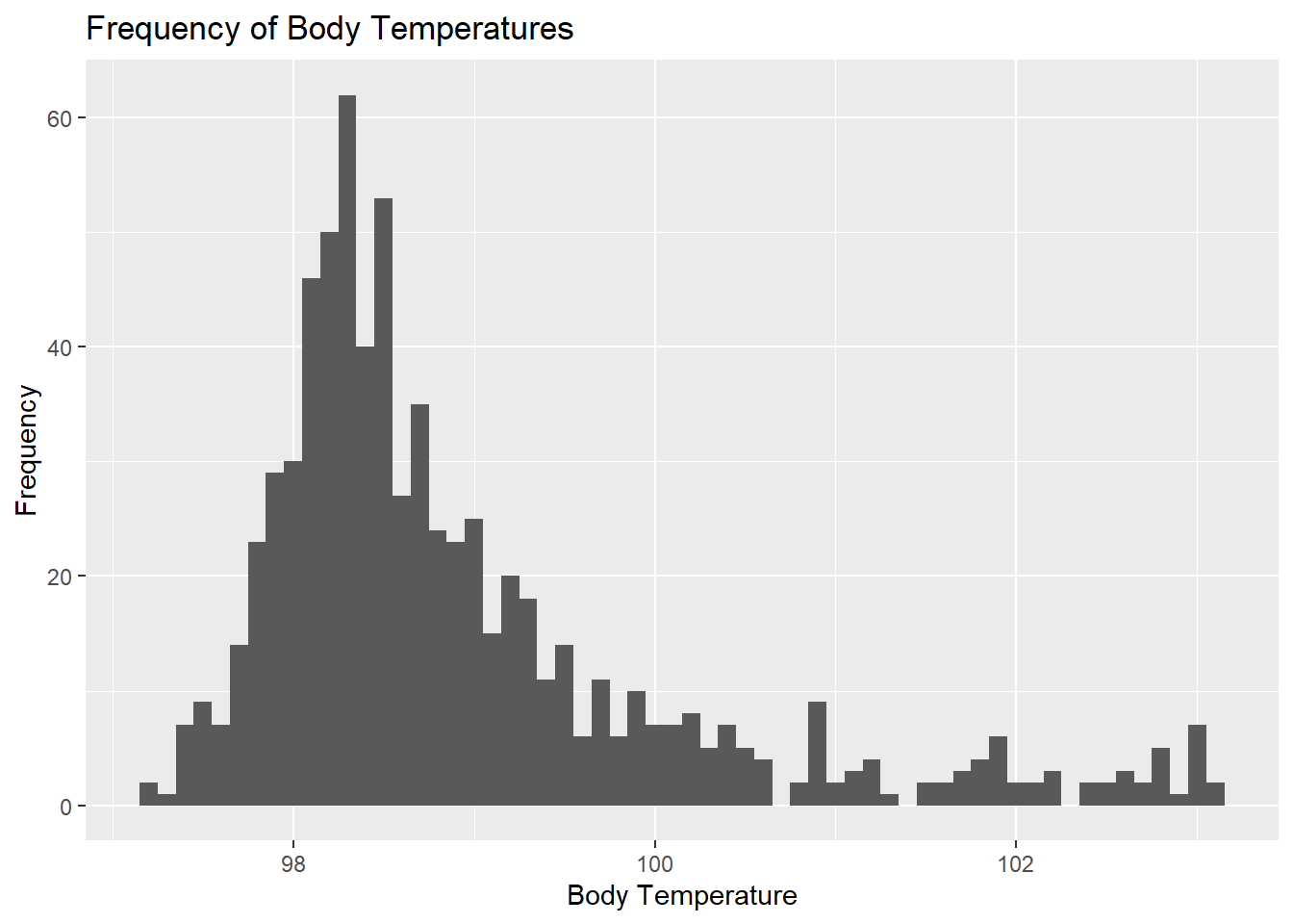

Data Visualization: Predictors and Outcomes

Selected Predictors of Interest for Outcome of Nausea: Headache, EarPn, Vomit

Selected Predictors of Interest for Outcome of Body Temperature: SwollenLymphNodes, SubjectiveFever, MyalgiaYN, Myalgia, ChillsSweats

Since it is difficult to represent categorical variables as themselves instead of numeric, I have decided to plot the Nausea variable as 0 for “No” and 1 for “Yes” on the y-axis.

Ear Pain vs Nausea

ggplot(clean_data %>% mutate(Nausea = if_else(Nausea == "Yes", 1, 0)), aes(x = EarPn, y = Nausea)) +
  geom_point() +
  geom_jitter() +
  geom_violin() +
  labs(x = "Ear Pain")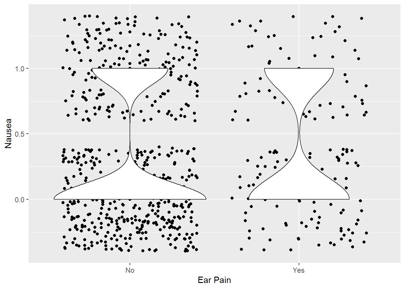

Most do not have ear pain. This violin plot also depicts greater lack of nausea for those who don’t have ear pain. For those that do, the frequency distributions seem relatively similar, though the frequency of “Yes” to ear pain still results in slightly fewer cases of nausea.

Vomit vs Nausea

ggplot(clean_data %>% mutate(Nausea = if_else(Nausea == "Yes", 1, 0)), aes(x = Vomit, y = Nausea)) + 
  geom_point() + 
  geom_jitter() +
  geom_violin() +
  labs(x = "Vomiting")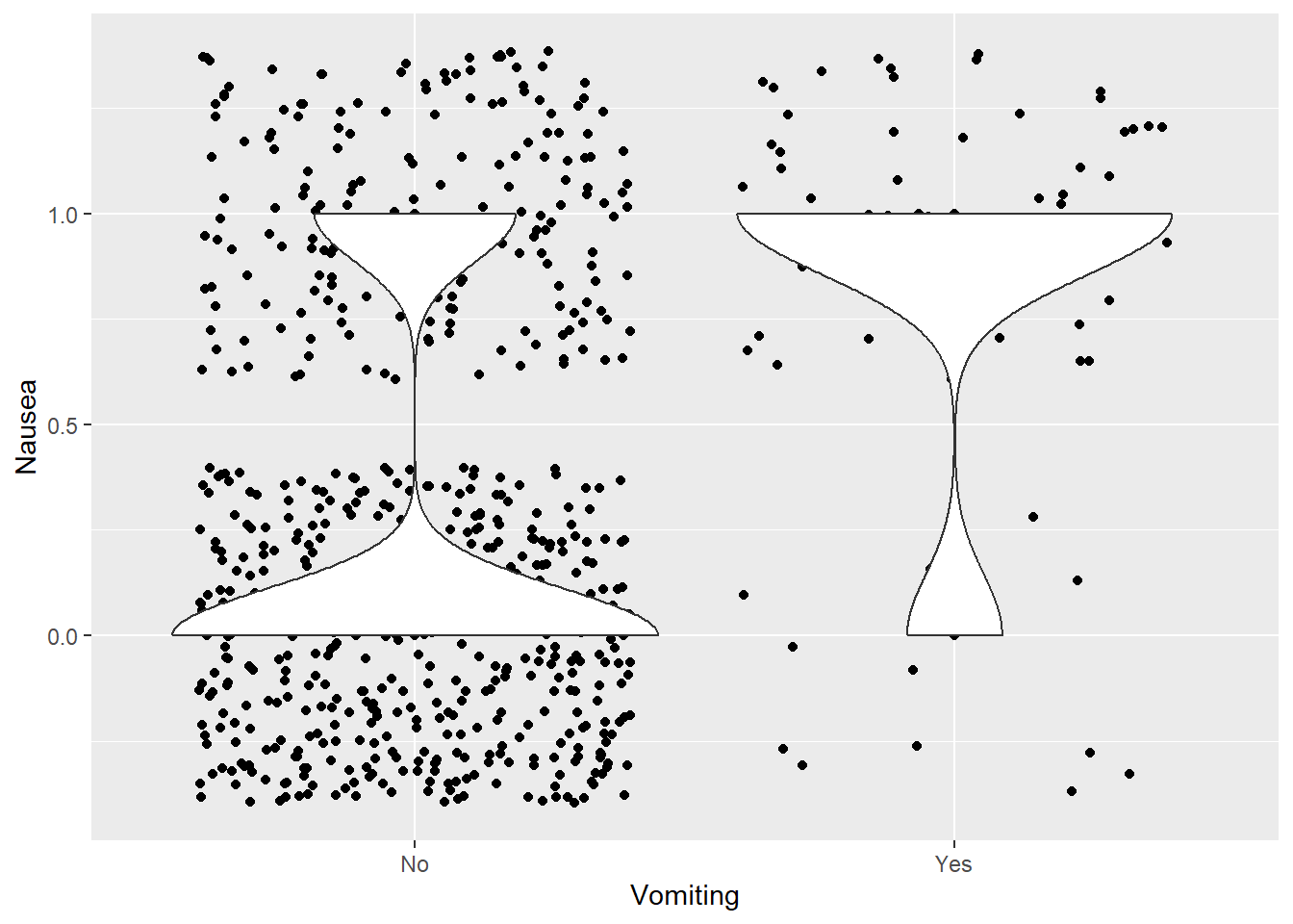

Most do not have vomiting. However, the violin plot above shows greater frequency of nausea with vomiting than vice-versa (which makes sense).

Headache vs Nausea

ggplot(clean_data %>% mutate(Nausea = if_else(Nausea == "Yes", 1, 0)), aes(x = Headache, y = Nausea)) + 
  geom_point() + 
  geom_jitter() +
  geom_violin()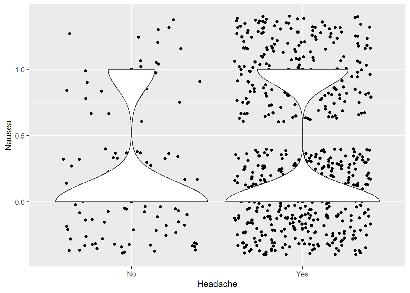

Most have a headache. From the violin graph, it appears that headache may influence nausea, though a statistical test or model should be done to verify this.

Subjective Fever vs Body Temperature

ggplot(clean_data, aes(x = SubjectiveFever, y = BodyTemp)) +
  geom_point() + geom_boxplot() +
  labs(x = "Subjective Fever", y = "Body Temperature")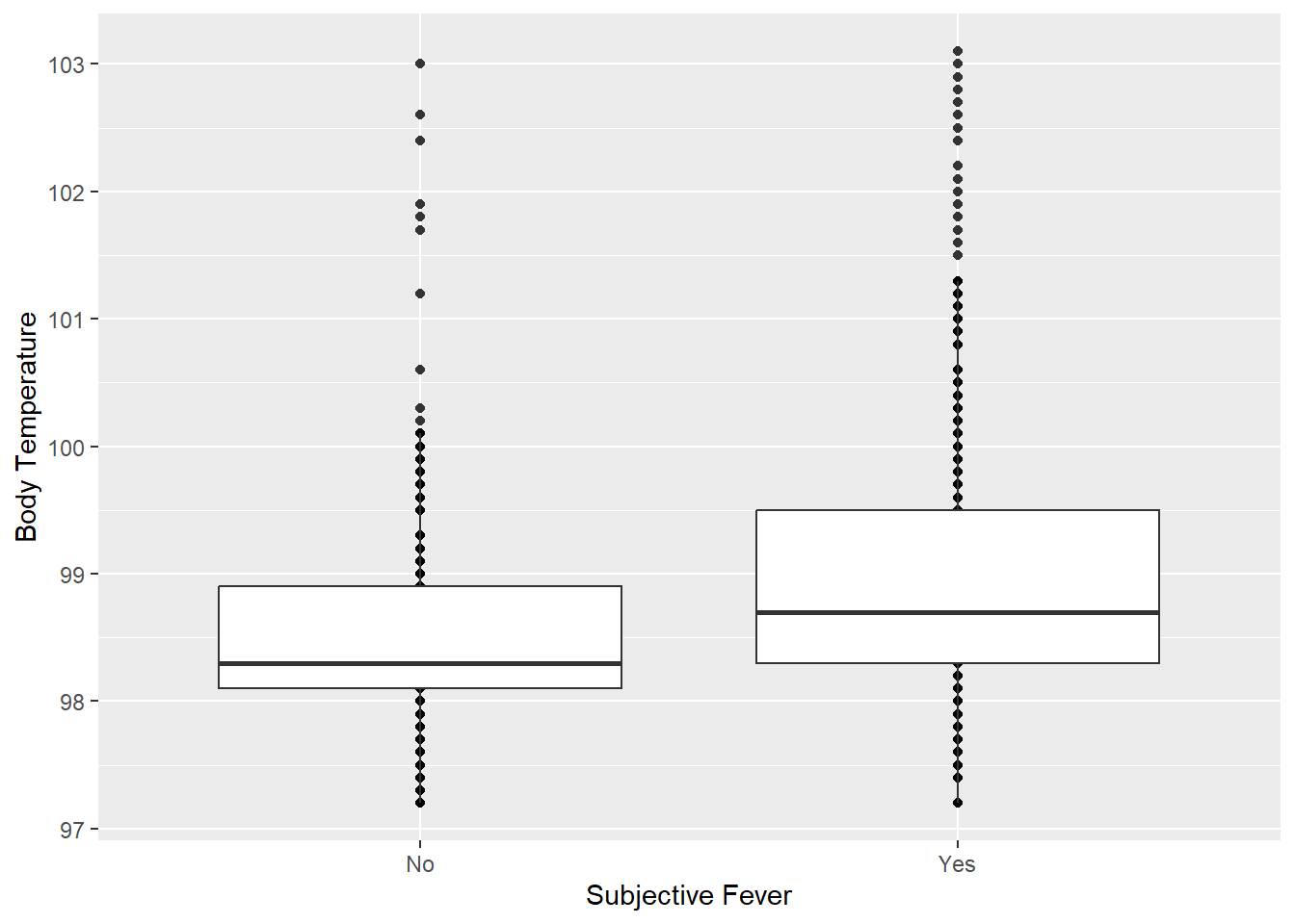

Those who say “Yes” to subjective fever tend to have higher body temperatures than those who say “No”.

Swollen Lymph Nodes vs Body Temperature

ggplot(clean_data, aes(x = SwollenLymphNodes, y = BodyTemp)) +
  geom_point() + geom_boxplot()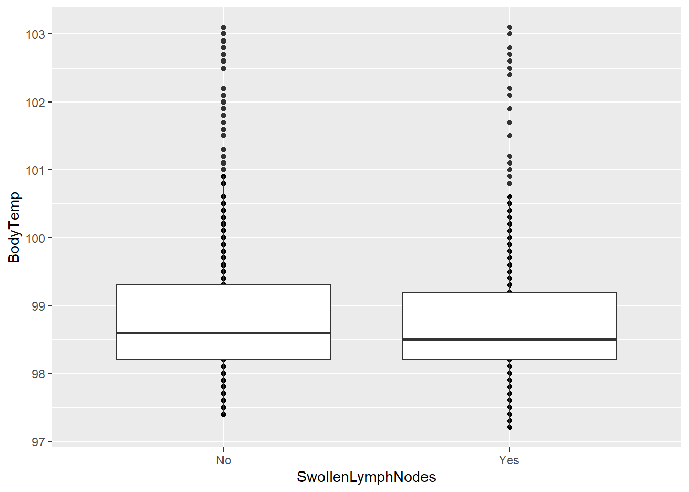

There appears to be little difference between the body temperatures of those who do have swollen lymph nodes and those who do not.

Myalgia vs Body Temperature

# Y/N
ggplot(clean_data, aes(x = MyalgiaYN, y = BodyTemp)) +
  geom_point() + geom_boxplot()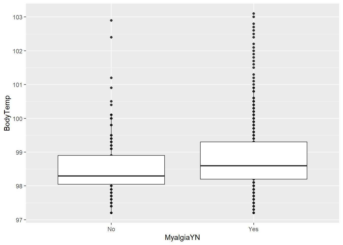

# Myalgia Severity
ggplot(clean_data, aes(x = Myalgia, y = BodyTemp)) +
  geom_point() + geom_boxplot()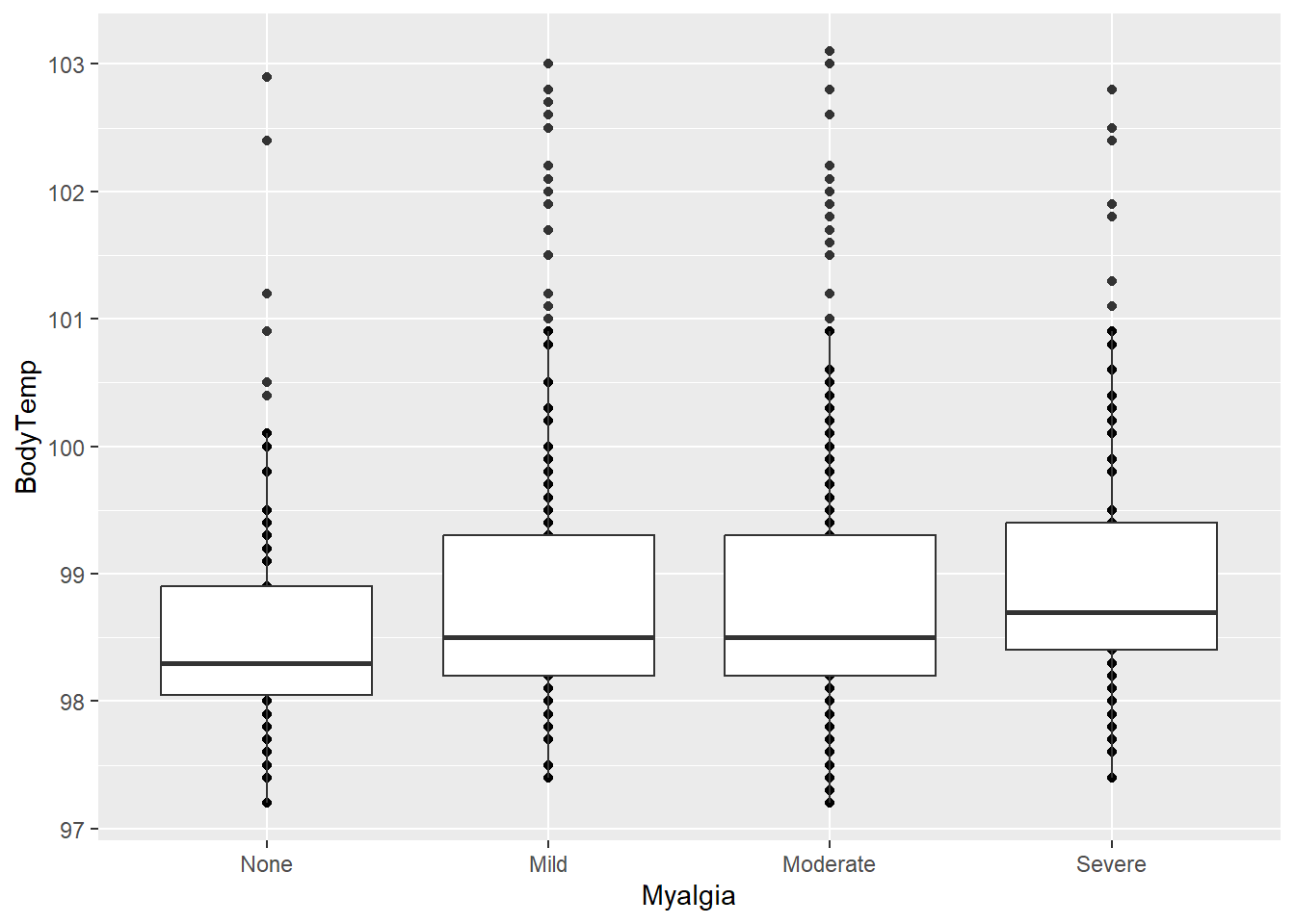

It seems that there is an association between having myalgia and a higher body temperature.

Chills/Sweats vs Body Temperature

ggplot(clean_data, aes(x = ChillsSweats, y = BodyTemp)) +
  geom_point() + 
  geom_boxplot() +
  labs(x = "Chills/Sweats")

From the boxplot, it appears that those with chills/sweats tend to have higher body temperatures than those without.