# Check the Help File for Gapminderhelp(gapminder)
starting httpd help server ... done
# Data Structurestr(gapminder)
'data.frame':   10545 obs. of  9 variables:
 $ country         : Factor w/ 185 levels "Albania","Algeria",..: 1 2 3 4 5 6 7 8 9 10 ...
 $ year            : int  1960 1960 1960 1960 1960 1960 1960 1960 1960 1960 ...
 $ infant_mortality: num  115.4 148.2 208 NA 59.9 ...
 $ life_expectancy : num  62.9 47.5 36 63 65.4 ...
 $ fertility       : num  6.19 7.65 7.32 4.43 3.11 4.55 4.82 3.45 2.7 5.57 ...
 $ population      : num  1636054 11124892 5270844 54681 20619075 ...
 $ gdp             : num  NA 1.38e+10 NA NA 1.08e+11 ...
 $ continent       : Factor w/ 5 levels "Africa","Americas",..: 4 1 1 2 2 3 2 5 4 3 ...
 $ region          : Factor w/ 22 levels "Australia and New Zealand",..: 19 11 10 2 15 21 2 1 22 21 ...
# Data Summarysummary(gapminder)
                country           year      infant_mortality life_expectancy
 Albania            :   57   Min.   :1960   Min.   :  1.50   Min.   :13.20
 Algeria            :   57   1st Qu.:1974   1st Qu.: 16.00   1st Qu.:57.50
 Angola             :   57   Median :1988   Median : 41.50   Median :67.54
 Antigua and Barbuda:   57   Mean   :1988   Mean   : 55.31   Mean   :64.81
 Argentina          :   57   3rd Qu.:2002   3rd Qu.: 85.10   3rd Qu.:73.00
 Armenia            :   57   Max.   :2016   Max.   :276.90   Max.   :83.90
 (Other)            :10203                  NA's   :1453
   fertility       population             gdp               continent
 Min.   :0.840   Min.   :3.124e+04   Min.   :4.040e+07   Africa  :2907
 1st Qu.:2.200   1st Qu.:1.333e+06   1st Qu.:1.846e+09   Americas:2052
 Median :3.750   Median :5.009e+06   Median :7.794e+09   Asia    :2679
 Mean   :4.084   Mean   :2.701e+07   Mean   :1.480e+11   Europe  :2223
 3rd Qu.:6.000   3rd Qu.:1.523e+07   3rd Qu.:5.540e+10   Oceania : 684
 Max.   :9.220   Max.   :1.376e+09   Max.   :1.174e+13
 NA's   :187     NA's   :185         NA's   :2972
             region
 Western Asia   :1026
 Eastern Africa : 912
 Western Africa : 912
 Caribbean      : 741
 South America  : 684
 Southern Europe: 684
 (Other)        :5586
# Classclass(gapminder)
[1] "data.frame"
Data Processing
# Assign African Countries to a New Objectafricadata <- gapminder %>%filter(continent =="Africa")## Find Missing Values in Infant Mortalityyears_of_na_infant_mortality <- africadata %>%select(year, infant_mortality) %>%filter(is.na(infant_mortality) ==TRUE) %>%group_by(year) %>%count()unique(years_of_na_infant_mortality$year)
# Checking New Object Structure and Summarystr(africadata)
'data.frame':   2907 obs. of  9 variables:
 $ country         : Factor w/ 185 levels "Albania","Algeria",..: 2 3 18 22 26 27 29 31 32 33 ...
 $ year            : int  1960 1960 1960 1960 1960 1960 1960 1960 1960 1960 ...
 $ infant_mortality: num  148 208 187 116 161 ...
 $ life_expectancy : num  47.5 36 38.3 50.3 35.2 ...
 $ fertility       : num  7.65 7.32 6.28 6.62 6.29 6.95 5.65 6.89 5.84 6.25 ...
 $ population      : num  11124892 5270844 2431620 524029 4829291 ...
 $ gdp             : num  1.38e+10 NA 6.22e+08 1.24e+08 5.97e+08 ...
 $ continent       : Factor w/ 5 levels "Africa","Americas",..: 1 1 1 1 1 1 1 1 1 1 ...
 $ region          : Factor w/ 22 levels "Australia and New Zealand",..: 11 10 20 17 20 5 10 20 10 10 ...
summary(africadata)
         country          year      infant_mortality life_expectancy
 Algeria     :  57   Min.   :1960   Min.   : 11.40   Min.   :13.20
 Angola      :  57   1st Qu.:1974   1st Qu.: 62.20   1st Qu.:48.23
 Benin       :  57   Median :1988   Median : 93.40   Median :53.98
 Botswana    :  57   Mean   :1988   Mean   : 95.12   Mean   :54.38
 Burkina Faso:  57   3rd Qu.:2002   3rd Qu.:124.70   3rd Qu.:60.10
 Burundi     :  57   Max.   :2016   Max.   :237.40   Max.   :77.60
 (Other)     :2565                  NA's   :226
   fertility       population             gdp               continent
 Min.   :1.500   Min.   :    41538   Min.   :4.659e+07   Africa  :2907
 1st Qu.:5.160   1st Qu.:  1605232   1st Qu.:8.373e+08   Americas:   0
 Median :6.160   Median :  5570982   Median :2.448e+09   Asia    :   0
 Mean   :5.851   Mean   : 12235961   Mean   :9.346e+09   Europe  :   0
 3rd Qu.:6.860   3rd Qu.: 13888152   3rd Qu.:6.552e+09   Oceania :   0
 Max.   :8.450   Max.   :182201962   Max.   :1.935e+11
 NA's   :51      NA's   :51          NA's   :637
                       region
 Eastern Africa           :912
 Western Africa           :912
 Middle Africa            :456
 Northern Africa          :342
 Southern Africa          :285
 Australia and New Zealand:  0
 (Other)                  :  0
# Making New Datasets for Infant Mortality + Life Expectancy (IMLE) & Population + Life Expectancy (PLE)IMLE <- africadata %>%select(infant_mortality, life_expectancy)PLE <- africadata %>%select(population, life_expectancy)# Checking IMLE and PLE Structure and Summaries## Structurestr(IMLE)
'data.frame':   2907 obs. of  2 variables:
 $ infant_mortality: num  148 208 187 116 161 ...
 $ life_expectancy : num  47.5 36 38.3 50.3 35.2 ...
str(PLE)
'data.frame':   2907 obs. of  2 variables:
 $ population     : num  11124892 5270844 2431620 524029 4829291 ...
 $ life_expectancy: num  47.5 36 38.3 50.3 35.2 ...
## Summarysummary(IMLE)
 infant_mortality life_expectancy
 Min.   : 11.40   Min.   :13.20
 1st Qu.: 62.20   1st Qu.:48.23
 Median : 93.40   Median :53.98
 Mean   : 95.12   Mean   :54.38
 3rd Qu.:124.70   3rd Qu.:60.10
 Max.   :237.40   Max.   :77.60
 NA's   :226
summary(PLE)
   population        life_expectancy
 Min.   :    41538   Min.   :13.20
 1st Qu.:  1605232   1st Qu.:48.23
 Median :  5570982   Median :53.98
 Mean   : 12235961   Mean   :54.38
 3rd Qu.: 13888152   3rd Qu.:60.10
 Max.   :182201962   Max.   :77.60
 NA's   :51
Graphing
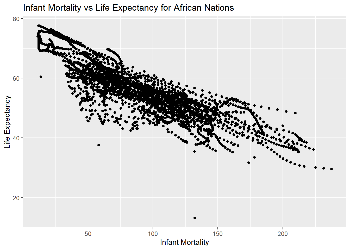
# IMLE: Infant Mortality vs Life Expectancyggplot(IMLE, aes(x = infant_mortality, y = life_expectancy)) +geom_point() +labs(x ="Infant Mortality", y ="Life Expectancy", title ="Infant Mortality vs Life Expectancy for African Nations")
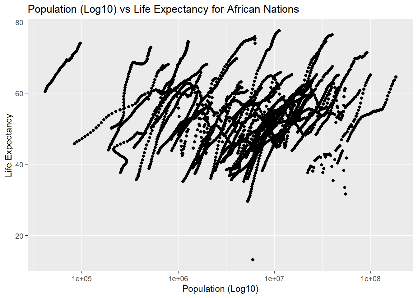
# PLEggplot(PLE, aes(x = population, y = life_expectancy)) +geom_point() +scale_x_log10() +labs(x ="Population (Log10)", y ="Life Expectancy", title ="Population (Log10) vs Life Expectancy for African Nations")
# Make New Object to House Year 2000 Datadata_2000 <- africadata %>%filter(year ==2000)# Check Structure and Summarystr(data_2000)
'data.frame':   51 obs. of  9 variables:
 $ country         : Factor w/ 185 levels "Albania","Algeria",..: 2 3 18 22 26 27 29 31 32 33 ...
 $ year            : int  2000 2000 2000 2000 2000 2000 2000 2000 2000 2000 ...
 $ infant_mortality: num  33.9 128.3 89.3 52.4 96.2 ...
 $ life_expectancy : num  73.3 52.3 57.2 47.6 52.6 46.7 54.3 68.4 45.3 51.5 ...
 $ fertility       : num  2.51 6.84 5.98 3.41 6.59 7.06 5.62 3.7 5.45 7.35 ...
 $ population      : num  31183658 15058638 6949366 1736579 11607944 ...
 $ gdp             : num  5.48e+10 9.13e+09 2.25e+09 5.63e+09 2.61e+09 ...
 $ continent       : Factor w/ 5 levels "Africa","Americas",..: 1 1 1 1 1 1 1 1 1 1 ...
 $ region          : Factor w/ 22 levels "Australia and New Zealand",..: 11 10 20 17 20 5 10 20 10 10 ...
summary(data_2000)
         country        year      infant_mortality life_expectancy
 Algeria     : 1   Min.   :2000   Min.   : 12.30   Min.   :37.60
 Angola      : 1   1st Qu.:2000   1st Qu.: 60.80   1st Qu.:51.75
 Benin       : 1   Median :2000   Median : 80.30   Median :54.30
 Botswana    : 1   Mean   :2000   Mean   : 78.93   Mean   :56.36
 Burkina Faso: 1   3rd Qu.:2000   3rd Qu.:103.30   3rd Qu.:60.00
 Burundi     : 1   Max.   :2000   Max.   :143.30   Max.   :75.00
 (Other)     :45
   fertility       population             gdp               continent
 Min.   :1.990   Min.   :    81154   Min.   :2.019e+08   Africa  :51
 1st Qu.:4.150   1st Qu.:  2304687   1st Qu.:1.274e+09   Americas: 0
 Median :5.550   Median :  8799165   Median :3.238e+09   Asia    : 0
 Mean   :5.156   Mean   : 15659800   Mean   :1.155e+10   Europe  : 0
 3rd Qu.:5.960   3rd Qu.: 17391242   3rd Qu.:8.654e+09   Oceania : 0
 Max.   :7.730   Max.   :122876723   Max.   :1.329e+11

                       region
 Eastern Africa           :16
 Western Africa           :16
 Middle Africa            : 8
 Northern Africa          : 6
 Southern Africa          : 5
 Australia and New Zealand: 0
 (Other)                  : 0
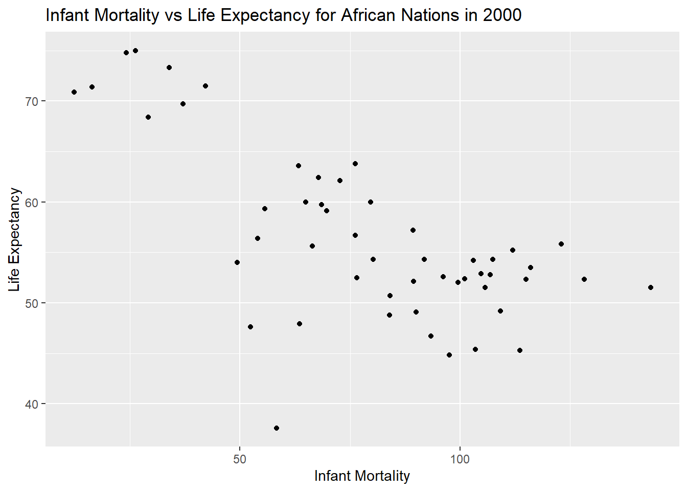
# Reevaluating Previous PlotsIMLE <- data_2000 %>%select(infant_mortality, life_expectancy)PLE <- data_2000 %>%select(population, life_expectancy)## IMLE: Infant Mortality vs Life Expectancyggplot(IMLE, aes(x = infant_mortality, y = life_expectancy)) +geom_point() +labs(x ="Infant Mortality", y ="Life Expectancy", title ="Infant Mortality vs Life Expectancy for African Nations in 2000")
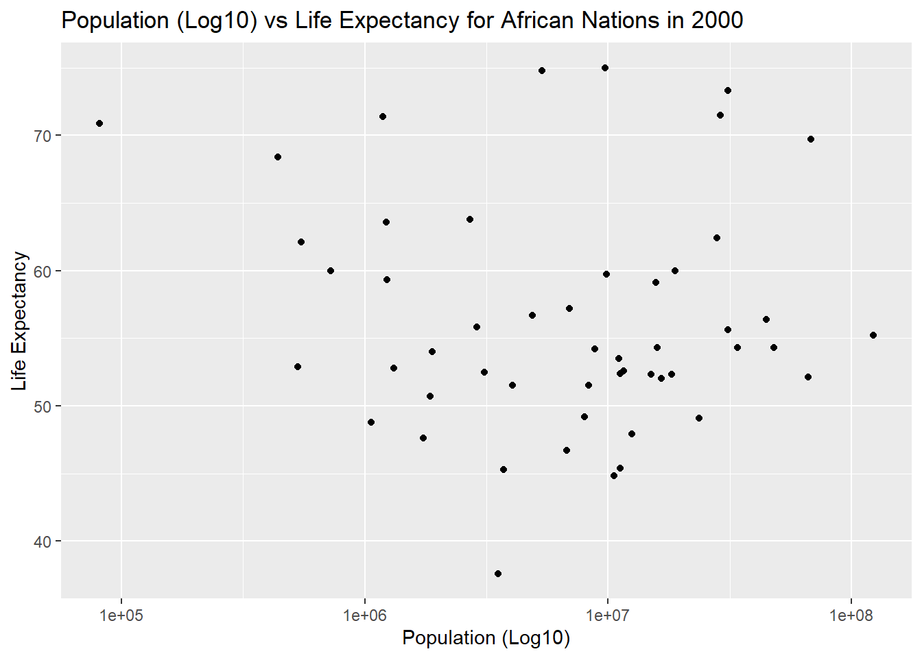
## PLEggplot(PLE, aes(x = population, y = life_expectancy)) +geom_point() +scale_x_log10() +labs(x ="Population (Log10)", y ="Life Expectancy", title ="Population (Log10) vs Life Expectancy for African Nations in 2000")
# Fitting a Simple Modelfit1 <-lm(life_expectancy ~ infant_mortality, data = data_2000)fit2 <-lm(life_expectancy ~ population, data = data_2000)# Summary of Modelssummary(fit1)
Call:
lm(formula = life_expectancy ~ infant_mortality, data = data_2000)

Residuals:
     Min       1Q   Median       3Q      Max
-22.6651  -3.7087   0.9914   4.0408   8.6817

Coefficients:
                 Estimate Std. Error t value Pr(>|t|)
(Intercept)      71.29331    2.42611  29.386  < 2e-16 ***
infant_mortality -0.18916    0.02869  -6.594 2.83e-08 ***
---
Signif. codes:  0 '***' 0.001 '**' 0.01 '*' 0.05 '.' 0.1 ' ' 1

Residual standard error: 6.221 on 49 degrees of freedom
Multiple R-squared:  0.4701,    Adjusted R-squared:  0.4593
F-statistic: 43.48 on 1 and 49 DF,  p-value: 2.826e-08
summary(fit2)
Call:
lm(formula = life_expectancy ~ population, data = data_2000)

Residuals:
    Min      1Q  Median      3Q     Max
-18.429  -4.602  -2.568   3.800  18.802

Coefficients:
             Estimate Std. Error t value Pr(>|t|)
(Intercept) 5.593e+01  1.468e+00  38.097   <2e-16 ***
population  2.756e-08  5.459e-08   0.505    0.616
---
Signif. codes:  0 '***' 0.001 '**' 0.01 '*' 0.05 '.' 0.1 ' ' 1

Residual standard error: 8.524 on 49 degrees of freedom
Multiple R-squared:  0.005176,  Adjusted R-squared:  -0.01513
F-statistic: 0.2549 on 1 and 49 DF,  p-value: 0.6159
According to the first model, infant mortality is a significant predictor (p < 0.001) on life expectancy for African nations. In contrast, population is not a significant predictor (p = 0.616) for life expectancy in the second model.
Hi! This section added by Katie Wells.
Continued analysis of the dataset
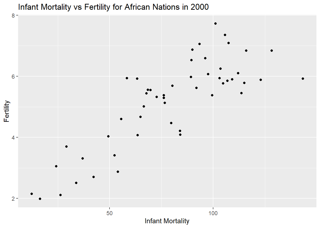
## Comparing fertility and infant mortality for the 2000 datasetggplot(data_2000, aes(x = infant_mortality, y = fertility)) +geom_point() +labs(x ="Infant Mortality", y ="Fertility", title ="Infant Mortality vs Fertility for African Nations in 2000")
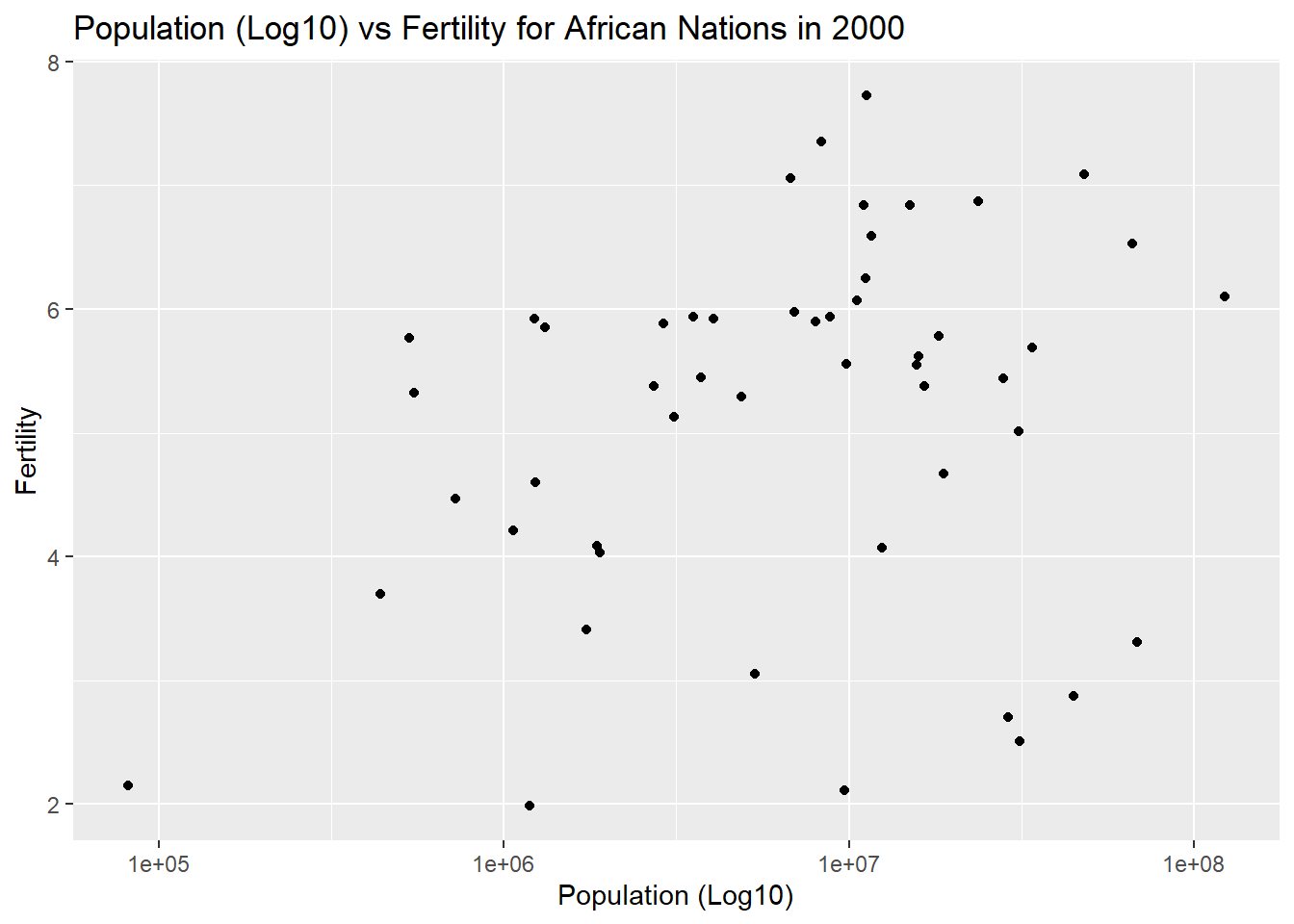
## Comparing population size and fertility for the 2000 datasetggplot(data_2000, aes(x = population, y = fertility)) +geom_point() +scale_x_log10() +labs(x ="Population (Log10)", y ="Fertility", title ="Population (Log10) vs Fertility for African Nations in 2000")
There appears to be a positive correlation between infant mortality and fertility but no strong correlation between fertility and population size.
## load packageslibrary("broom")
## Fitting fertility against population and infant mortality in a linear modelfit3 <-lm(fertility ~ population, data = data_2000)fit4 <-lm(fertility ~ infant_mortality, data = data_2000)## show fit output as a tabletidy(fit3)
# A tibble: 2 × 5
  term             estimate     std.error statistic  p.value
  <chr>               <dbl>         <dbl>     <dbl>    <dbl>
1 (Intercept) 5.09          0.253            20.1   2.43e-25
2 population  0.00000000447 0.00000000939     0.476 6.36e- 1
The fit of first model shows that infant mortality is a significant predictor (p < 0.001) on fertility for African nations. In contrast, population is not a significant predictor (p = 0.064) for fertility in the second model.