Module 10 Exercise: Flu Analysis Modeling Workflow

Flu Analysis (Logistic Regression) Model Evaluation, Performed by Kai Chen

Load Libraries

# Pathing
library(here)

here() starts at C:/Users/Kai/Documents/School/Colleges/UGA/MPH Year/Spring 2023/Modern Data Analysis/kaichen-MADA-portfolio

# Data Handling
library(tidyverse)

── Attaching packages
───────────────────────────────────────
tidyverse 1.3.2 ──

✔ ggplot2 3.4.0      ✔ purrr   1.0.1 
✔ tibble  3.1.8      ✔ dplyr   1.0.10
✔ tidyr   1.2.1      ✔ stringr 1.5.0 
✔ readr   2.1.3      ✔ forcats 0.5.2 
── Conflicts ────────────────────────────────────────── tidyverse_conflicts() ──
✖ dplyr::filter() masks stats::filter()
✖ dplyr::lag()    masks stats::lag()

# Model Handling and Evaluation
library(tidymodels)

── Attaching packages ────────────────────────────────────── tidymodels 1.0.0 ──
✔ broom        1.0.3     ✔ rsample      1.1.1
✔ dials        1.1.0     ✔ tune         1.0.1
✔ infer        1.0.4     ✔ workflows    1.1.2
✔ modeldata    1.0.1     ✔ workflowsets 1.0.0
✔ parsnip      1.0.3     ✔ yardstick    1.1.0
✔ recipes      1.0.4     
── Conflicts ───────────────────────────────────────── tidymodels_conflicts() ──
✖ scales::discard() masks purrr::discard()
✖ dplyr::filter()   masks stats::filter()
✖ recipes::fixed()  masks stringr::fixed()
✖ dplyr::lag()      masks stats::lag()
✖ yardstick::spec() masks readr::spec()
✖ recipes::step()   masks stats::step()
• Dig deeper into tidy modeling with R at https://www.tmwr.org

Load Data

# Set Variable for Where Original Data is Located
data_location <- here("fluanalysis", "data", "cleaned_data.rds")

# Read in Original Data
original_data <- readRDS(data_location)

Data Splitting

# Set Seed for Reproducible Analysis
set.seed(2023)

# Split Original Data into Training and Testing Data
data_split <- initial_split(original_data, prop = 3/4)

# Create Data Frames from Split Data
train_data <- training(data_split)
test_data <- testing(data_split)

Workflow Creation and Model Fitting

Create Recipe for Fitting Logistic Model (Categorical Outcome)

flu_recipe <- recipe(Nausea ~ ., data = train_data)

Workflow to Create Logistic Model

# Set Model to Logistic Regression
logistic_regression_model <- logistic_reg() %>% set_engine("glm")

# Specifying Workflow
logistic_workflow <- workflow() %>% 
  add_model(logistic_regression_model) %>%
  add_recipe(flu_recipe)

# Fitting/Training
logistic_fit <- logistic_workflow %>%
  fit(data = train_data)

Model 1 Evaluation

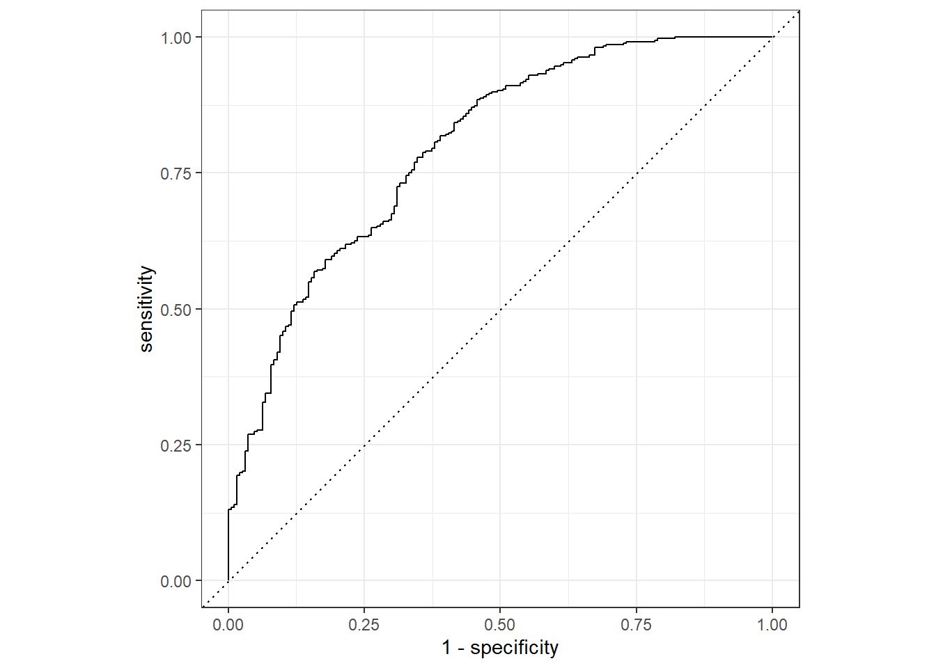
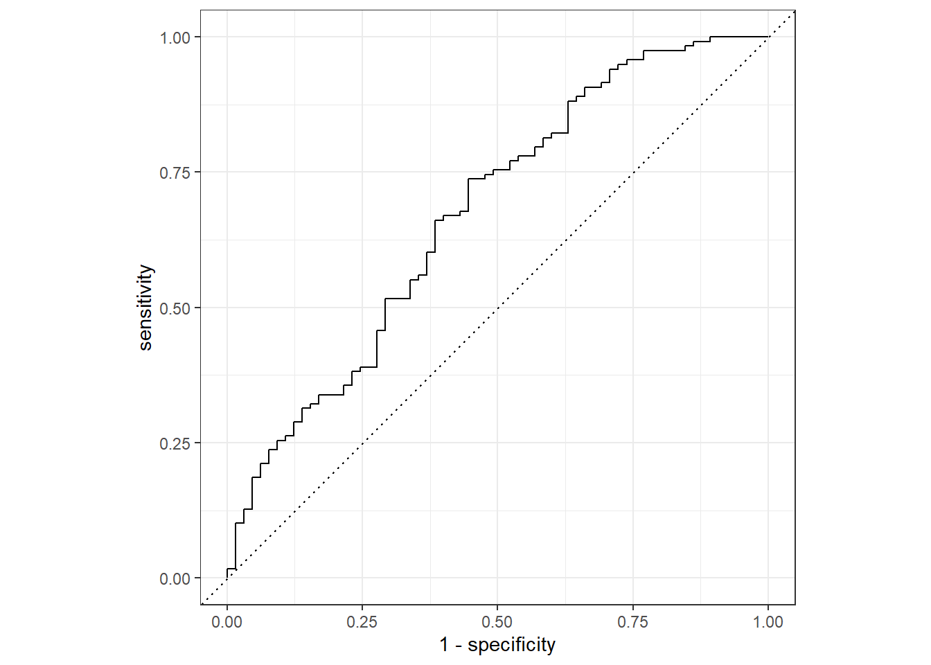
Prediction + ROC Curve

# Training Data
predict(logistic_fit, train_data)

Warning in predict.lm(object, newdata, se.fit, scale = 1, type = if (type == :
prediction from a rank-deficient fit may be misleading

# A tibble: 547 × 1
   .pred_class
   <fct>      
 1 No         
 2 No         
 3 No         
 4 No         
 5 No         
 6 No         
 7 No         
 8 No         
 9 Yes        
10 No         
# … with 537 more rows

train_augment <- augment(logistic_fit, train_data)

Warning in predict.lm(object, newdata, se.fit, scale = 1, type = if (type == :
prediction from a rank-deficient fit may be misleading

Warning in predict.lm(object, newdata, se.fit, scale = 1, type = if (type == :
prediction from a rank-deficient fit may be misleading

## Generate ROC Curve
train_augment %>% 
  roc_curve(truth = Nausea, .pred_No) %>%
  autoplot()

## Calculate ROC-AUC
train_augment %>%
  roc_auc(truth = Nausea, .pred_No)

# A tibble: 1 × 3
  .metric .estimator .estimate
  <chr>   <chr>          <dbl>
1 roc_auc binary         0.796

# Test Data
predict(logistic_fit, test_data)

Warning in predict.lm(object, newdata, se.fit, scale = 1, type = if (type == :
prediction from a rank-deficient fit may be misleading

# A tibble: 183 × 1
   .pred_class
   <fct>      
 1 Yes        
 2 No         
 3 No         
 4 Yes        
 5 No         
 6 Yes        
 7 No         
 8 Yes        
 9 No         
10 No         
# … with 173 more rows

test_augment <- augment(logistic_fit, test_data)

Warning in predict.lm(object, newdata, se.fit, scale = 1, type = if (type == :
prediction from a rank-deficient fit may be misleading

Warning in predict.lm(object, newdata, se.fit, scale = 1, type = if (type == :
prediction from a rank-deficient fit may be misleading

## Generate ROC Curve
test_augment %>%
  roc_curve(truth = Nausea, .pred_No) %>%
  autoplot()

## Calculate ROC-AUC
test_augment %>%
  roc_auc(truth = Nausea, .pred_No)

# A tibble: 1 × 3
  .metric .estimator .estimate
  <chr>   <chr>          <dbl>
1 roc_auc binary         0.672

The fitted model appears to perform worse on the test data (ROC-AUC = 0.672) than on the training data (ROC-AUC = 0.796).

Alternative Model (Single Predictor: RunnyNose)

Modified Flu Recipe

new_flu_recipe <- recipe(Nausea ~ RunnyNose, data = train_data)

New Workflow

# Specifying Workflow
new_logistic_workflow <- workflow() %>% 
  add_model(logistic_regression_model) %>%
  add_recipe(new_flu_recipe)

# Fitting/Training
new_logistic_fit <- new_logistic_workflow %>%
  fit(data = train_data)

Alternative Model Evaluation

# Training Data
predict(new_logistic_fit, train_data)

# A tibble: 547 × 1
   .pred_class
   <fct>      
 1 No         
 2 No         
 3 No         
 4 No         
 5 No         
 6 No         
 7 No         
 8 No         
 9 No         
10 No         
# … with 537 more rows

new_train_augment <- augment(new_logistic_fit, train_data)
## Generate ROC Curve
new_train_augment %>% 
  roc_curve(truth = Nausea, .pred_No) %>%
  autoplot()

## Calculate ROC-AUC
new_train_augment %>%
  roc_auc(truth = Nausea, .pred_No)

# A tibble: 1 × 3
  .metric .estimator .estimate
  <chr>   <chr>          <dbl>
1 roc_auc binary         0.515

# Test Data
predict(new_logistic_fit, test_data)

# A tibble: 183 × 1
   .pred_class
   <fct>      
 1 No         
 2 No         
 3 No         
 4 No         
 5 No         
 6 No         
 7 No         
 8 No         
 9 No         
10 No         
# … with 173 more rows

new_test_augment <- augment(new_logistic_fit, test_data)
## Generate ROC Curve
new_test_augment %>%
  roc_curve(truth = Nausea, .pred_No) %>%
  autoplot()

## Calculate ROC-AUC
new_test_augment %>%
  roc_auc(truth = Nausea, .pred_No)

# A tibble: 1 × 3
  .metric .estimator .estimate
  <chr>   <chr>          <dbl>
1 roc_auc binary         0.476

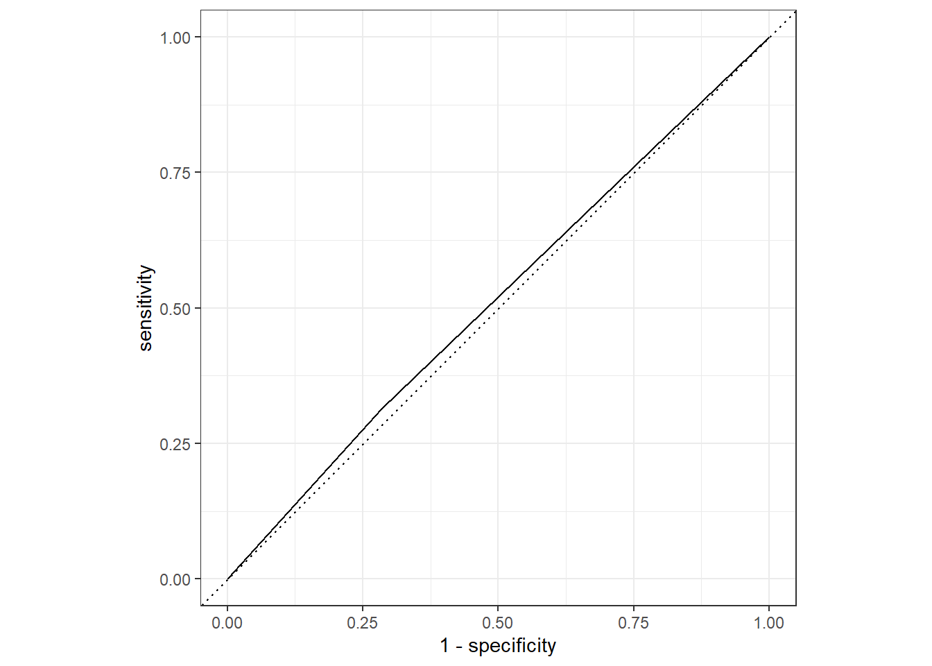
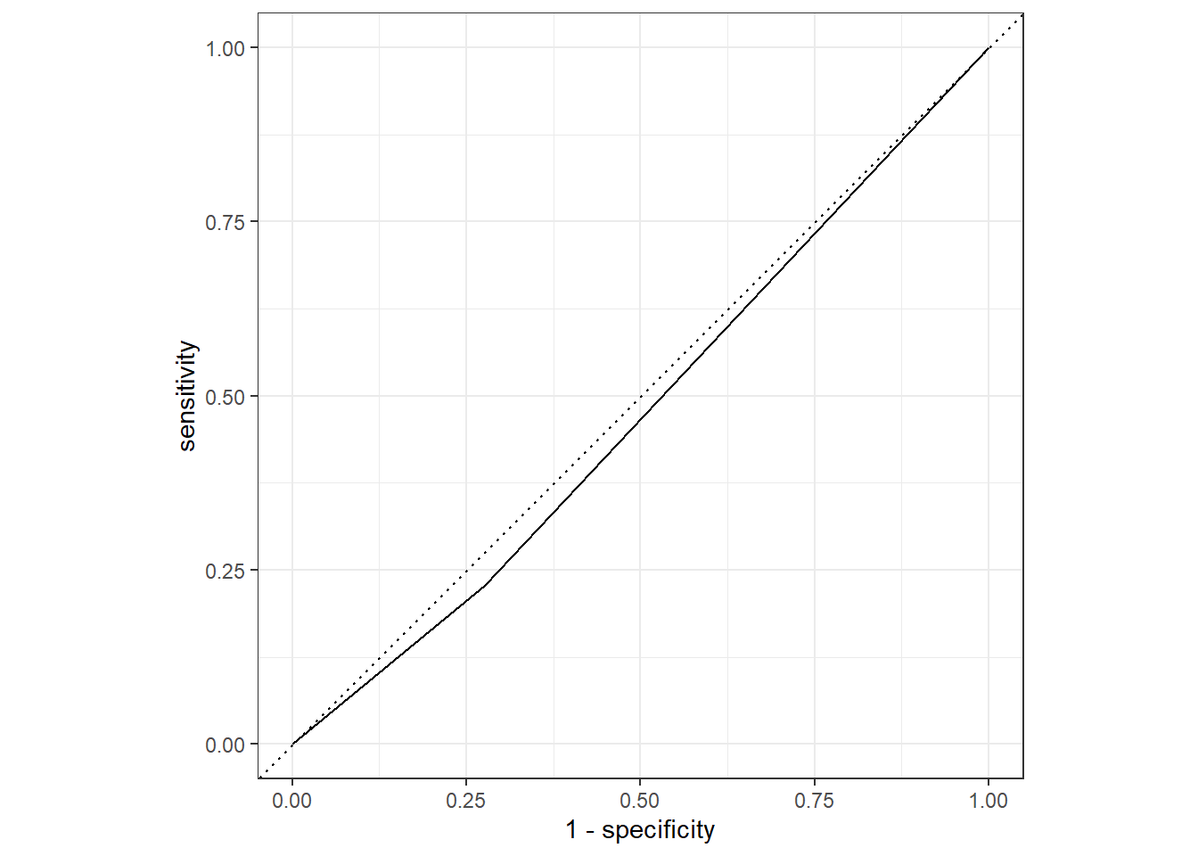
The alternative model that uses just one predictor appears to be much worse (Training ROC-AUC: 0.515, Test ROC-AUC: 0.476) than the model that uses all predictors (Training ROC-AUC: 0.796, Test ROC-AUC: 0.672).

This section added by CONNOR H ROSS (below)

Part II: Continous Outcome

# Part II: Continous Outcome
## Libraries already loaded above (Thanks Kailin :))

## Set seed for reproducibility
set.seed(2)



## Split 3/4 of the data into the training set
flu_splitc1 <- initial_split(original_data, prop = 3/4)



## Create data frame for the two sets:
train_datac1 <- training(flu_splitc1)
test_datac1 <- testing(flu_splitc1)


## Full model

### Creating my recipe
flu_recipec1 <- recipe(BodyTemp ~ ., data = original_data)



### Prepare model
lin_modc1 <- linear_reg() %>%
  set_engine("lm")



### Create workflow
flu_wflowc1 <- workflow() %>%
  add_model(lin_modc1) %>%
  add_recipe(flu_recipec1)



### Prepare the recipe and train the model
flu_fitc1 <- flu_wflowc1 %>%
  fit(data = train_datac1)



### Tidy output
flu_fitc1 %>%
  extract_fit_parsnip() %>%
  tidy()

# A tibble: 38 × 5
   term                 estimate std.error statistic  p.value
   <chr>                   <dbl>     <dbl>     <dbl>    <dbl>
 1 (Intercept)           98.2        0.351   280.    0       
 2 SwollenLymphNodesYes  -0.100      0.109    -0.923 0.356   
 3 ChestCongestionYes     0.0519     0.117     0.441 0.659   
 4 ChillsSweatsYes        0.163      0.151     1.08  0.282   
 5 NasalCongestionYes    -0.239      0.132    -1.82  0.0698  
 6 CoughYNYes             0.141      0.271     0.522 0.602   
 7 SneezeYes             -0.310      0.116    -2.67  0.00784 
 8 FatigueYes             0.197      0.185     1.06  0.288   
 9 SubjectiveFeverYes     0.476      0.124     3.83  0.000147
10 HeadacheYes            0.0282     0.151     0.187 0.852   
# … with 28 more rows

### Prediction
predict(flu_fitc1, test_datac1)

Warning in predict.lm(object = object$fit, newdata = new_data, type =
"response"): prediction from a rank-deficient fit may be misleading

# A tibble: 183 × 1
   .pred
   <dbl>
 1  99.6
 2  99.8
 3  99.8
 4  98.4
 5  98.7
 6  98.6
 7  98.9
 8  99.0
 9  99.7
10  99.3
# … with 173 more rows

### Augment
flu_augc1 <- augment(flu_fitc1, test_datac1)

Warning in predict.lm(object = object$fit, newdata = new_data, type =
"response"): prediction from a rank-deficient fit may be misleading

### Looks like
flu_augc1 %>%
  select(BodyTemp, .pred)

# A tibble: 183 × 2
   BodyTemp .pred
      <dbl> <dbl>
 1    100.   99.6
 2     98.2  99.8
 3     97.9  99.8
 4     98.1  98.4
 5     99.2  98.7
 6     98.1  98.6
 7     98.5  98.9
 8    100.   99.0
 9     98.9  99.7
10     98.8  99.3
# … with 173 more rows

### flu_aug
flu_augc1 %>%
  rmse(BodyTemp , .pred)

# A tibble: 1 × 3
  .metric .estimator .estimate
  <chr>   <chr>          <dbl>
1 rmse    standard        1.15

### One Predictor
## Creating my recipe2
flu_recipec2 <- recipe(BodyTemp ~ RunnyNose, data = original_data)



#### Previous model will work



### Create workflow2
flu_wflowc2 <- workflow() %>%
  add_model(lin_modc1) %>%
  add_recipe(flu_recipec2)



### Prepare the recipe and train the model2
flu_fitc2 <- flu_wflowc2 %>%
  fit(data = train_datac1)



### Tidy output2
flu_fitc2 %>%
  extract_fit_parsnip() %>%
  tidy()

# A tibble: 2 × 5
  term         estimate std.error statistic p.value
  <chr>           <dbl>     <dbl>     <dbl>   <dbl>
1 (Intercept)    99.2      0.0968   1024.   0      
2 RunnyNoseYes   -0.366    0.114      -3.21 0.00139

### Prediction2
predict(flu_fitc2, test_datac1)

# A tibble: 183 × 1
   .pred
   <dbl>
 1  99.2
 2  99.2
 3  99.2
 4  98.8
 5  98.8
 6  98.8
 7  98.8
 8  98.8
 9  99.2
10  99.2
# … with 173 more rows

### Augment2
flu_augc2 <- augment(flu_fitc2, test_datac1)



### Looks like2
flu_augc2 %>%
  select(BodyTemp, .pred)

# A tibble: 183 × 2
   BodyTemp .pred
      <dbl> <dbl>
 1    100.   99.2
 2     98.2  99.2
 3     97.9  99.2
 4     98.1  98.8
 5     99.2  98.8
 6     98.1  98.8
 7     98.5  98.8
 8    100.   98.8
 9     98.9  99.2
10     98.8  99.2
# … with 173 more rows

### flu_aug2
flu_augc2 %>%
  rmse(BodyTemp , .pred)

# A tibble: 1 × 3
  .metric .estimator .estimate
  <chr>   <chr>          <dbl>
1 rmse    standard        1.18

^^ This section added by CONNOR H ROSS ^^